Decoding the Circuits: Track Analysis
Not all racetracks are created equal. A car that dominates the high-speed straights of Monza might struggle in the tight, winding corners of Monaco. Our goal was to create a data-driven classification system. We treated each circuit as a complex dataset, engineering its geometric layout to uncover distinct families of tracks using unsupervised machine learning.
Data Preprocessing
The foundation of this analysis was built on raw geospatial data from Tomo Bacinger’s GeoJSON circuit database. The initial pipeline focused on transforming this raw data into meaningful metrics:
- Coordinate Transformation: Raw latitude/longitude coordinates for each track were converted into a 2D Cartesian plane (x, y meters) to allow for accurate geometric calculations
- Curvature Calculation: Using numerical derivatives (`np.gradient`), we calculated the point-by-point curvature along each track. This metric is crucial as it quantifies how sharply the track turns at any given point
- Track Feature Extraction: From the curvature and coordinate data, we engineered four key metrics to serve as each circuit's unique feature signature:
- Percent Straights: The percentage of the track with near-zero curvature, representing full-throttle sections
- Average Absolute Curvature: The mean intensity of all turns on the track
- Number of Corners: A count of distinct cornering events on a lap
- Standard Deviation of Curvature: A measure of corner variety. A high value indicates a mix of slow hairpins and fast sweepers, while a low value suggests more uniform corners
ML Algorithms / Models Implemented
We explored two primary unsupervised clustering algorithms to group the circuits based on their characteristics. The goal was to see if the data would naturally form intuitive families without any prior labels.
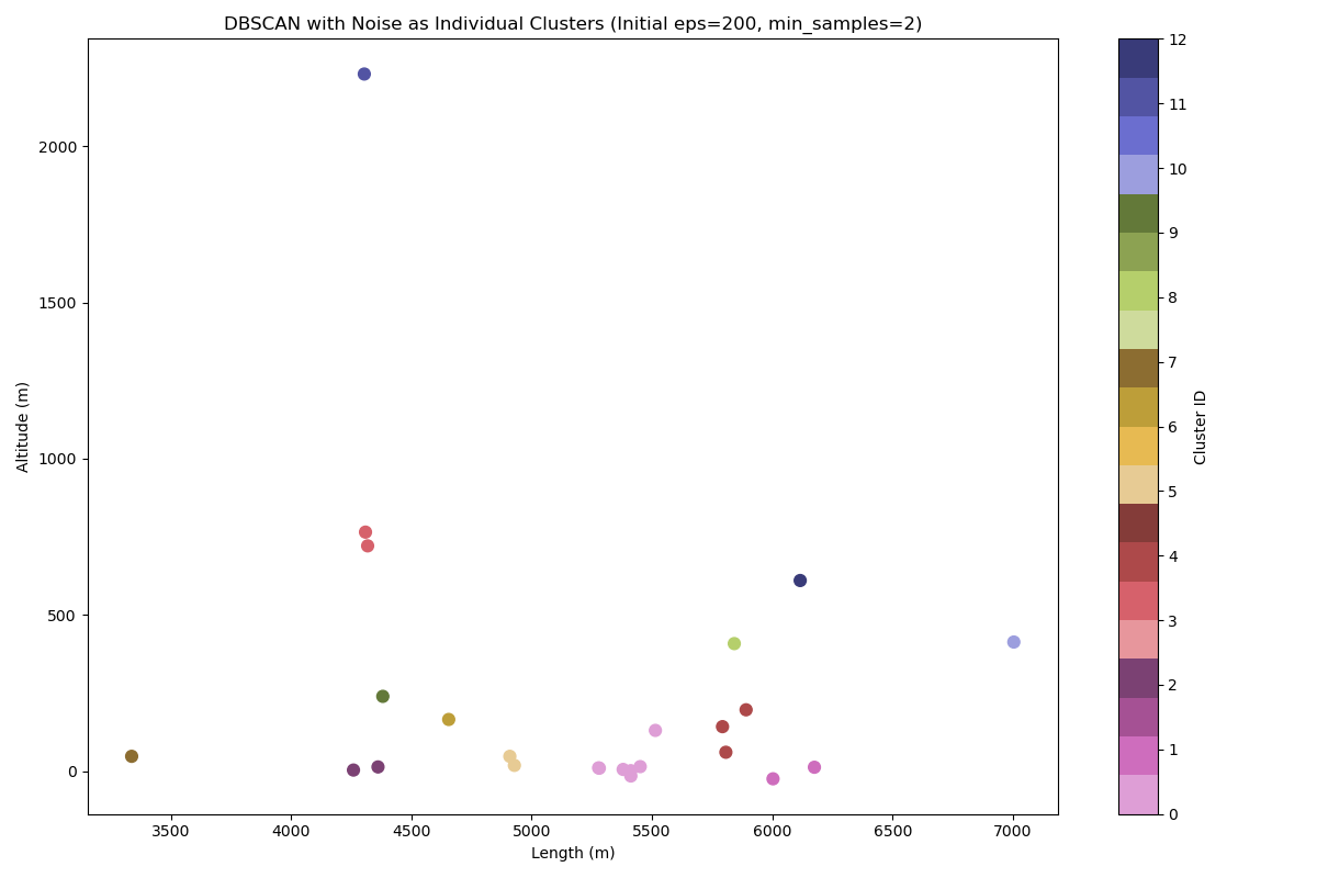
DBSCAN: Density-Based Clustering
We first applied DBSCAN to the simplest features: track length and altitude. This model identifies clusters by finding high-density regions in the data. A unique modification was made to our implementation: instead of marking isolated tracks as "noise," each noise point was assigned its own unique cluster ID. This ensures every track is categorized, either as part of a larger group or as a unique outlier.
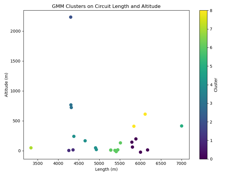
Gaussian Mixture Model (GMM): Probabilistic Clustering
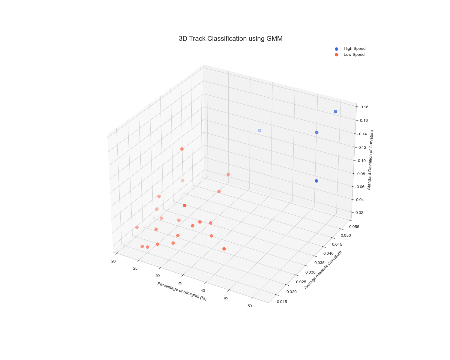
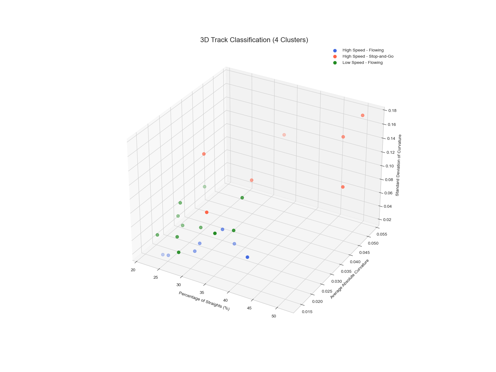
Our primary modeling approach used a GMM, a powerful probabilistic algorithm. Unlike DBSCAN, which makes hard assignments, GMM assigns each track a probability of belonging to several different clusters. Our most advanced model used a **4-component GMM** applied to the four engineered "DNA" features
Benefits & Drawbacks
| Gaussian Mixture Model (GMM) | DBSCAN |
|---|---|
| Advantages | |
|
|
| Drawbacks | |
|
|
Quantitative Metrics
| Model | Features | Silhouette Score | Davies-Bouldin Index |
|---|---|---|---|
| GMM (2 Clusters) | Curvature-based | 0.494 | 0.698 |
| GMM (4 Clusters) | Curvature-based | 0.324 | 0.935 |
| DBSCAN | Altitude & Length | 0.477 | 0.215 |
Final Model Analysis
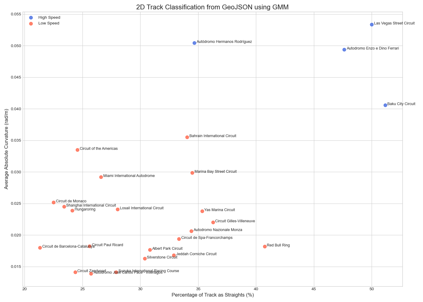
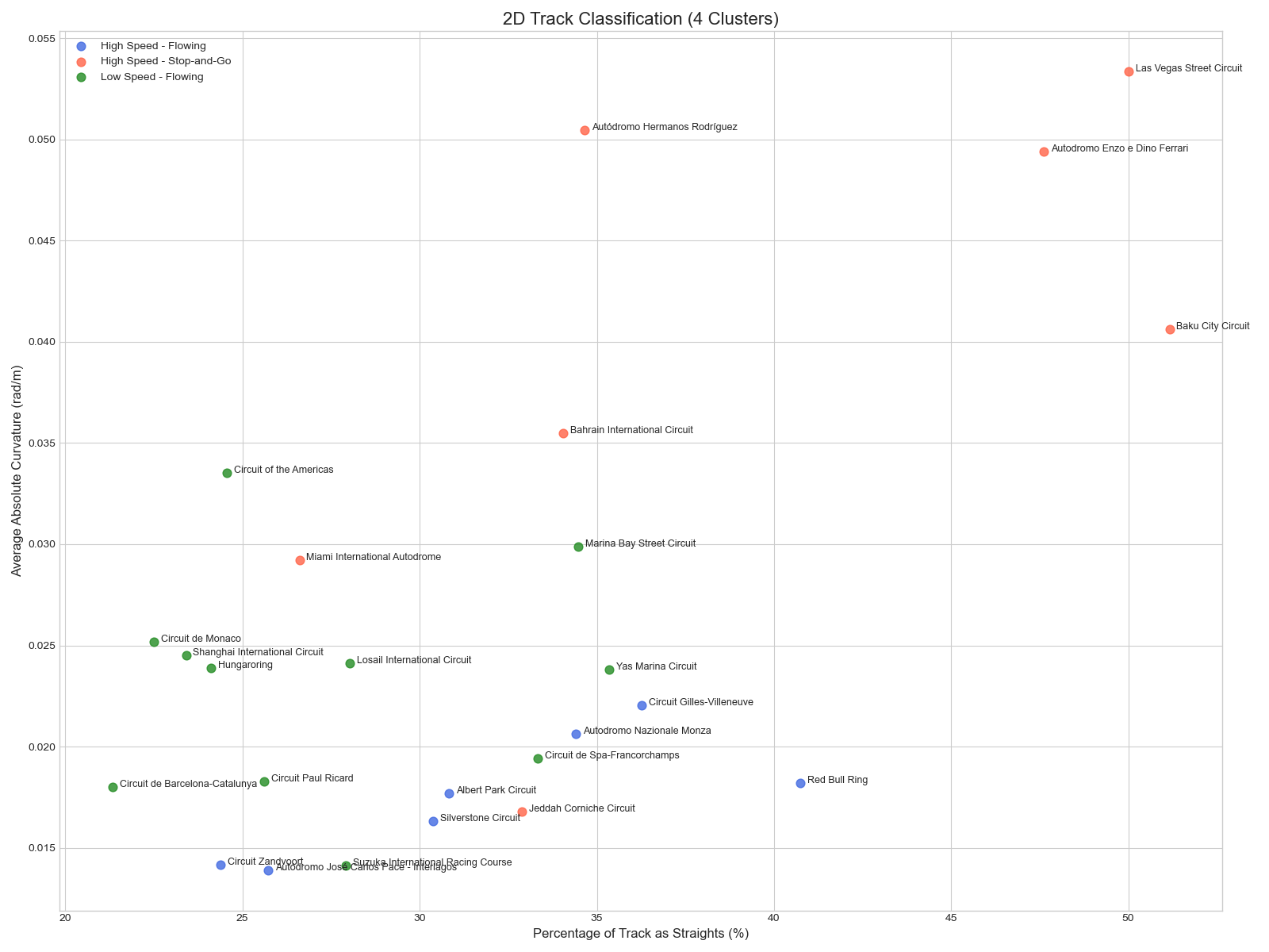
The GMM applied to our engineered features yielded the most insightful results. While a simple 2-cluster GMM produced the most mathematically distinct groups (highest Silhouette Score), the **4-cluster GMM** allowed us to create a richer, more strategically valuable classification system. We interpreted these four clusters by analyzing their average feature values, creating a 2x2 matrix of track archetypes:
- A track is classified as "High Speed" if its `percent_straights` is above the median, and "Low Speed" if below
- A track is classified as "Flowing" if its `std_curvature` is low (uniform corners), and "Stop-and-Go" if high (varied corners)
This resulted in four intuitive archetypes: High Speed - Flowing (e.g., Monza, Silverstone), High Speed - Stop-and-Go (e.g., Baku, Las Vegas), Low Speed - Flowing (e.g., Zandvoort), and Low Speed - Stop-and-Go (e.g., Monaco, Singapore). This classification, derived directly from the code's logic, provides a powerful framework for anticipating car performance and race strategy.
The 2‑cluster GMM yields the highest silhouette (0.494), cleanly splitting “High Speed” vs “Low Speed” circuits. Expanding to 4 GMM clusters provides richer archetypes (flowing vs stop‑and‑go) at the cost of separation. DBSCAN achieves the best Davies‑Bouldin (0.215), isolating outliers and grouping mid‑density tracks effectively, but requires fine‐tuned parameters. Overall, combining insights from both approaches gives the most complete picture of each track’s DNA.